8 Machine Learning Algorithms Explained in Human Language

What we call Machine Learning or Machine Learning is nothing other than the encounter of statistics with the computing power available today (memory, processors, graphics cards). This field has become very important because of the digital revolution in businesses, which has led to the production of massive data of various forms and types,

Bruno

What we call Machine Learning or Machine Learning is none other than the encounter of statistics with the computing power available today (memory, processors, graphics cards) .This field has become very important because of the digital revolution in companies, which has led to the production of massive data of various forms and types, at constantly increasing rates: Big Data.On a purely mathematical level, most of the algorithms used are already several decades old. In this article I will explain how 8 machine learning algorithms work in the simplest possible terms.

1. Some Main Concepts Before Tackling Algorithms

A. Classification or Prediction?

Classification

Assigning a class/category to each of the observations in a data set is a classification. This is done later, once the data is recovered.Example: Classification of reasons for consumers to visit stores in order to create a hyperpersonalized marketing campaign.

Prediction

A prediction is made based on a new observation. When it comes to a numerical variable (continuous) we speak of regression.Example: Prediction of a stroke based on electro-cardiogram data.

B. Supervised and unsupervised learning

Supervised

You already have labels on historical data and you are looking to classify new data. The number of classes is known.Example: In botany you have carried out measurements (length of the stem, petals,...) on 100 plants of 3 different species. Each of the measurements is labeled with the species of the plant. You want to build a model that will automatically be able to tell which species a new plant belongs to based on the same type of measurements.

Unsupervised

On the contrary, in unsupervised learning, you have no labels, no predefined classes. You want to identify common patterns in order to form homogeneous groups based on your observations.Example: You want to classify your customers according to their browsing history on your website but you did not create groups at first glance and are in an exploratory process to see what would be the groups of similar customers (behavioral marketing). In these cases a clustering algorithm (partitioning) is adapted.

2. Machine Learning Algorithms

We are going to describe 8 algorithms used in Machine Learning. The objective here is not to go into detail about the models but rather to give the reader elements of understanding about each of them.

A. “The Decision Tree”

A decision tree is used to classify future observations given a corpus of observations that are already labeled. This is the case of our botanical example where we already have 100 observations classified into species A, B and C. The tree starts with a root (where we have all our observations) then a series of branches whose intersections are called nodes and ends with leaves that each corresponds to one of the classes to be predicted. Tree depth is referred to as the maximum number of knots before reaching a leaf. Each node in the tree represents a rule (example: petal length greater than 2.5 cm). Browsing the tree is therefore checking a series of rules. The tree is built in such a way that each node corresponds to the rule (type of measurement and threshold) that will best divide the set of initial observations.Example:

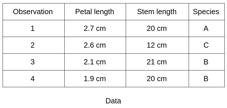
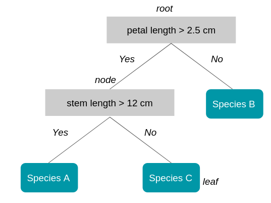
The tree has a depth of 2 (one node plus the root). The length of the petal is the first measure that is used because it best separates the 4 observations according to class membership (here to class B).

B. “Random Forests”

As the name suggests, the random forest algorithm is based on decision trees. To better understand the benefits and functioning of this algorithm, let's start with an example:You are looking for a good travel destination for your next vacation. You ask your best friend for his opinion. He asks you questions about your previous trips and makes a recommendation. You decide to ask a group of friends who ask you questions randomly. They each give you a recommendation. The destination selected is the one that was recommended the most by your friends. The recommendations made by your best friend and the group will both seem like good destination choices. But when the first recommendation method works very well for you, the second will be more reliable for you, the second will be more reliable for you, the second will be more reliable for you, the second will be more reliable for other people.This comes from the fact that your best friend, who builds a decision tree to give you a destination recommendation, knows you very well what caused the decision tree to over-learn about you (we talk about overfitting: over learning) .Your group of friends represents the random forest of multiple decision trees and it is a model, when used properly, avoid the pitfall of overfitting.

So how is this forest built?

Here are the main steps:

We take an X number of observations from the initial data set (with delivery).
We take a number K of the M available variables (features), for example: only temperature and population density
A decision tree is trained on this data set.
Steps 1. to 4 are repeated. Do not times so to obtain N trees.

For a new observation whose class we are looking for, we go down the N trees. Each tree offers a different class. The class selected is the one that is most represented among all the trees in the forest. (Majority vote/'together' in English).

C. The “Gradient Boosting”/“XG Boost”

The gradient boosting method is used to reinforce a model that produces weak predictions, for example a decision tree (see how to judge the quality of a model) .We will explain the principle of gradient boosting with the decision tree but it could be with another model. You have an individual database with demographic information and past activities. 50% of individuals are their age but the other half is unknown.You want to obtain the age of a person according to their activities: food shopping, television, television, gardening, gardening, gardening, video games... You choose a decision tree as a model, in this case it is a regression tree, in this case it is a regression tree, in this case it is a regression tree because the value to be predicted is numeric.Your first regression tree is satisfactory but largely perfected: it predicts, for example, that an individual is a regression tree, for example, that an individual is 19 years old when in reality he At 13, and Another 55 years old instead of 68. The principle of gradient boosting is that you are going to redo a model on the difference between the predicted value and the true value to be predicted.Age Prediction Tree 1 Difference Prediction Tree 21319-6156855+1363We will repeat this step N times where N is determined by successively minimizing the error between the prediction and the true value.The method to optimize is the method of descending the gradient that we will not explain here.The XG Boost (eXtreme Gradient Boosting) model is one of the implementations of gradient boosting founded by Tianqi Chen and has seduced the Kaggle data scientist community with its efficiency and performance. The publication explaining the algorithm can be found Hather.

D. “Genetic Algorithms”

As their name suggests, genetic algorithms are based on the process of genetic evolution that made us who we are... More prosaically, they are mainly used when we do not have initial observations and when we rather want a machine to learn as it tries. These algorithms are not the most effective for a specific problem, but rather for a set of sub-problems (for example, learning balance and walking in robotics).) .Let's take a simple example: We want to find the code for a safe which is made up of 15 letters: “MACHINELEARNING” The genetic algorithm approach will be as follows: We start from a population of 10,000 “chromosomes” of 15 letters each. We say to ourselves that the code is a word or a set of similar words. “DEEP-LEARNING” “STATISTICAL-INFERENCE” “INTERFACE-HUMAN-MACHINE” etc.We will define a method of reproduction: for example combining the beginning of one chromosome with the end of another.Ex: “DEEP-LEARNING” + “STATISTICAL-INFERENCE” + “STATISTICAL-INFERENCE” + “STATISTICAL-INFERENCE” + “STATISTICAL-INFERENCE” = “DEEP-INFERENCE” + “STATISTICAL-INFERENCE” = “DEEP-INFERENCE” + “STATISTICAL-INFERENCE” = “DEEP-INFERENCE” + “DEEP-INFERENCE” + “STATISTICAL-INFERENCE” = “DEEP-INFERENCE” + “STATISTICAL-INFERENCE” = “DEEP-INFERENCE” A method of mutation which makes it possible to evolve a progeny that is blocked. In our case it could be causing one of the letters to vary randomly. Finally, we define a score that will reward this or that chromosome progeny. In our case where the code is hidden we can imagine a sound that the chest would make when 80% of the letters are similar and that would become louder and louder as we get closer to the right code. Our genetic algorithm will start from the initial population and form chromosomes until the solution has been found.

E. The “Support Vector Machines”

Also known as an “SVM” (Support Vector Machine), this algorithm is mainly used for classification problems, although it has been extended to regression problems (Drucker et al., 96) .Let's go back to our example of ideal vacation destinations. For the simplicity of our example, let's consider only 2 variables to describe each city: temperature and population density. We can therefore represent cities in 2 dimensions. We represent by circles the cities that you liked to visit and by squares those that you liked less. When considering new cities you want to know which group is this city closest to. As we can see on the graph on the right there are numerous planes (lines when we only have 2 dimensions) that separate the two groups.

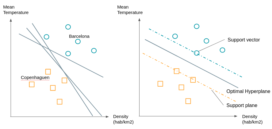
We will choose the line that has the maximum distance between the two groups. To build it we already see that we don't need all the points, we just have to take the points that are at the border of their group we call these points or vectors, the support vectors. The planes passing through these support vectors are called support planes. The separation plane will be the one that is equidistant from the two support planes. What if the groups are not as easily separable, for example on one of the dimensions of the circles are found in the squares and vice versa? We are going to transform these points by a function to be able to separate them. As in the example below:

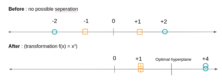
The SVM algorithm will therefore consist in looking for both the optimal hyperplane and in minimizing classification errors.

F. The “K Closest Neighbors”

Pause. After 5 relatively technical models, the K nearest neighbors algorithm will seem like a formality to you. Here's how it works:

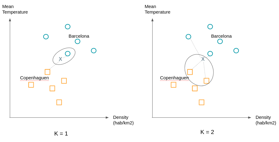
An observation is assigned the class of its K closest neighbors. “Is that all?!” You will tell me. Yes that's all, only as the following example shows the choice of K can change a lot of things. We will therefore try to try different values of K to obtain the most satisfactory separation.

G. “Logistic Regression”

First, let's recall the principle of linear regression. Linear regression is used to predict a numerical variable, for example the price of cotton according to other numerical or binary variables: the number of hectares that can be cultivated, the demand for cotton from various industries etc.It is a question of finding the coefficients a1, a2,... to have the best estimation:Cotton price = a1 * Number of hectares + a2 * Demand for cotton +... Logistic regression is used in classification in the same way as the algorithms exposed up to here. We will summarize the example of trips by considering only two classes: good destination (Y=1) and bad destination (Y=0).P (1): Probability the city is a good destination.P (0): Probability that the city is a bad destination.The city is represented by a number of variables, we are only going to consider two of them: temperature and population density.X = (X1: temperature, X2: population density) So we are interested in constructing a function that gives us for a city X:P (1|X): Probability that the destination is good knowing X, which is the same as saying probability that the city verifying X is a good destination. We would like to relate this probability to a linear combination such as a linear regression. Only the probability P (1|X) varies between 0 and 1 and we want a function that goes through the whole domain of real numbers (from -infinity to +infinity). For this we will start by considering P (1|X)/(1 — P (1|X)) which is the ratio between the probability that the destination is good and that the destination is bad. For high probabilities this ratio approaches + infinity (for example a probability of 0.99 gives 0.99/0.01 = 99) and for low probabilities it approaches 0: (a probability of 0.01 gives 0.01/0.99 = 0.0101) .We went from [0.1] to [0, +infinity [. To extend the 'scope' of possible values to] -infinity, [0] we take the natural logarithm of this ratio.It follows that we are looking for b0, 1b, b2,... such as:ln (P (1|X)/(1 — P (1|X)) = b0 + B1x1 + b2x2The right part represents the regression and the natural logarithm denotes the logistical part.The regression algorithm Denote the logistic part. Logistics will therefore find the best coefficients to minimize the error between the prediction made for the destinations visited and the true label (good, bad) given.

H. “Clustering”

Supervised vs unsupervised learning. Do you remember it? So far we have supervised exposed learning algorithms. The classes are known and we want to classify or predict a new observation. But what do you do when there is no predefined group? When you are just looking to find patterns shared by groups of individuals? Through their unsupervised learning, clustering algorithms fulfill this role. Let's take the example of a company that has begun its digital transformation. It has new sales and communication channels through its site and one or more associated mobile applications. In the past, it addressed its customers based on demographics and purchase history. But how can you use the navigation data of its customers? Does online behavior correspond to traditional customer segments? These questions can motivate the use of clustering to see if major trends are emerging. This makes it possible to disprove or confirm business intuitions that you may have. There are many clustering algorithms (hierarchical clustering, k-means, DBSCAN,...). One of the most used is the k-means algorithm. We will explain how it works simply: Even if we do not know how the clusters will be formed, the k-means algorithm requires giving the expected number of clusters. Techniques exist to find the optimal number of clusters. Consider the example of cities. Our data set has 2 variables, so we are using 2 dimensions. After an initial study we expect to have 2 clusters. We start by randomly placing two points; they represent our starting 'means'. We associate the observations closest to these means to the same clusters. Then we calculate the average of the observations of each cluster and move the means to the calculated position. We reassign the observations to the nearest means and so on.

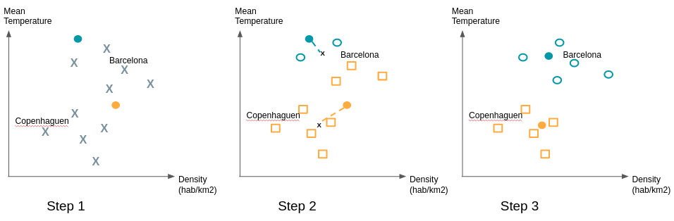
To ensure the stability of the groups found, it is recommended to repeat the drawing of the initial 'means' multiple times because some initial draws can give a configuration different from the vast majority of cases.

3. Factors of relevance and quality of machine learning algorithms

Machine learning algorithms are evaluated on the basis of their ability to classify or predict correctly both on the observations that were used to train the model (training and test game) but also and especially on observations whose label or value is known and which were not used in developing the model (validation game). Properly classifying implies both placing the observations in the right group and at the same time not Do not place them in the wrong groups. The metric chosen may vary depending on the intent of the algorithm and its business use. Several factors related to data can play a major role in the quality of algorithms. Here are the main ones:

A. The number of observations

The fewer observations there are, the more difficult the analysis is. But the more there are, the higher the need for computer memory and the longer the analysis takes).

B. The number and quality of attributes describing these observations

The distance between two numerical variables (price, size, weight, weight, weight, weight, light intensity, noise intensity, etc.) is easy to establish.
The one between two categorical attributes (color, beauty, utility...) is more delicate.

C. Percentage of completed and missing data

D. The “noise”

The number and the “location” of doubtful values (potential errors, outliers...) or naturally non-conforming to the general distribution pattern of the “examples” on their distribution space will impact on the quality of the analysis.

Conclusion

We saw that machine learning algorithms were used for two things: classifying and predicting and that they were divided into supervised and unsupervised algorithms. There are many possible algorithms, we went through 8 of them including logistic regression and random forests to classify an observation and clustering to make homogeneous groups emerge from the data. We also saw that the value of an algorithm depended on the associated cost or loss function but that its predictive power depended on several factors related to the quality and volume of data. I hope that this article gave you some elements of understanding about what is called “Machine Learning.” Do not hesitate to use the comment section to give me feedback on aspects that you would like to clarify or deepen.

Author

Gaël BonnardotCofounder and CTO at DataKeenAt Datakeen we seek to simplify the use and understanding of new algorithmic techniques by business functions in all industries.